Update 2:
Make sure you check out the successor of this project - Meccano Rubik’s Shrine, it’s even more awesome!
Update:
Since this post was published, we upgraded the scanner on the machine, and now the scanning process takes way less time. Check out the Hardware section.
TL;DR
For those who don’t feel like reading any further, here are some links:
- Project page on Meccano Kinematics website
- Solving algorithm implementation: GitHub
- Final video: YouTube
- Other Wilbert’s machines: YouTube channel
- More about Meccano and FAC system: Meccano Kinematics
Introduction
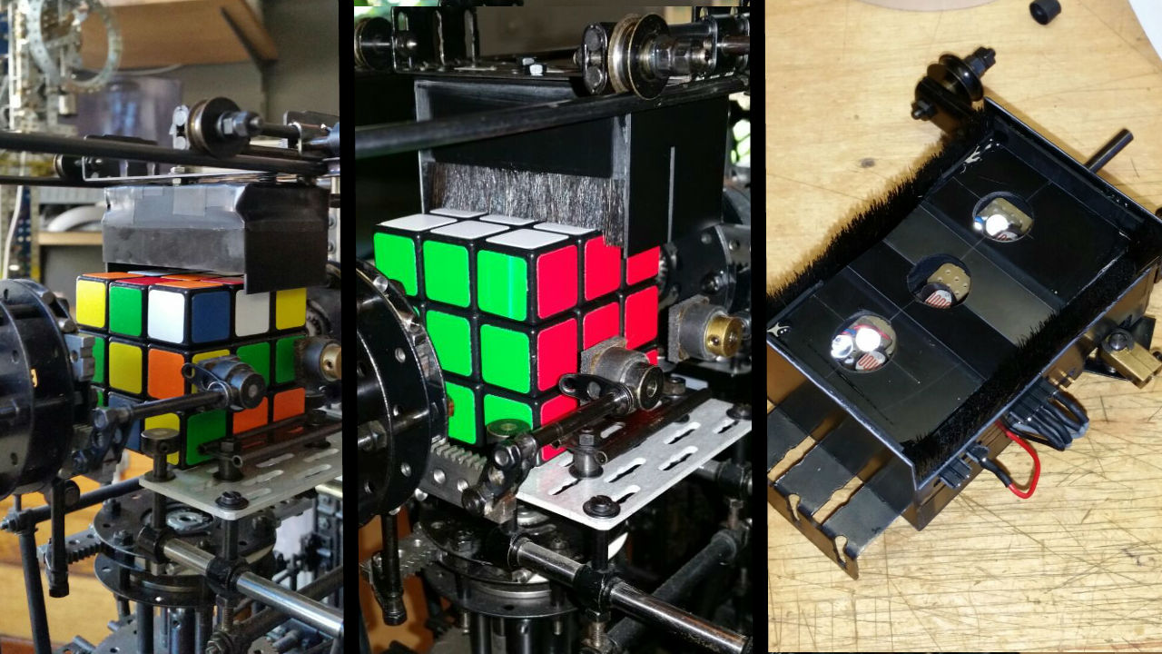
About three months ago I was introduced to Wilbert Swinkels. Normally you don’t meet people with such an amazing blend of skills and passion for creating awesomeness, so this was a great luck for me when he offered to help him with the Rubik’s cube solving machine.
The machine looked absolutely marvelous. Just like all other Wilbert’s creations, it is a piece of art by itself. Besides, color cubes had already carried me away once. With no doubt, I accepted his offer.
By the time I met Wilbert, he had been working on the machine for almost five years. It is quite an interesting story, with a number of great successes, disappointing failures, and invaluable experience. When I started working on it, most of the hardware-related problems had already been solved. There was even a proof-of-concept program for Arduino that could control grippers and scanner. However, the software part essentially did not exist.
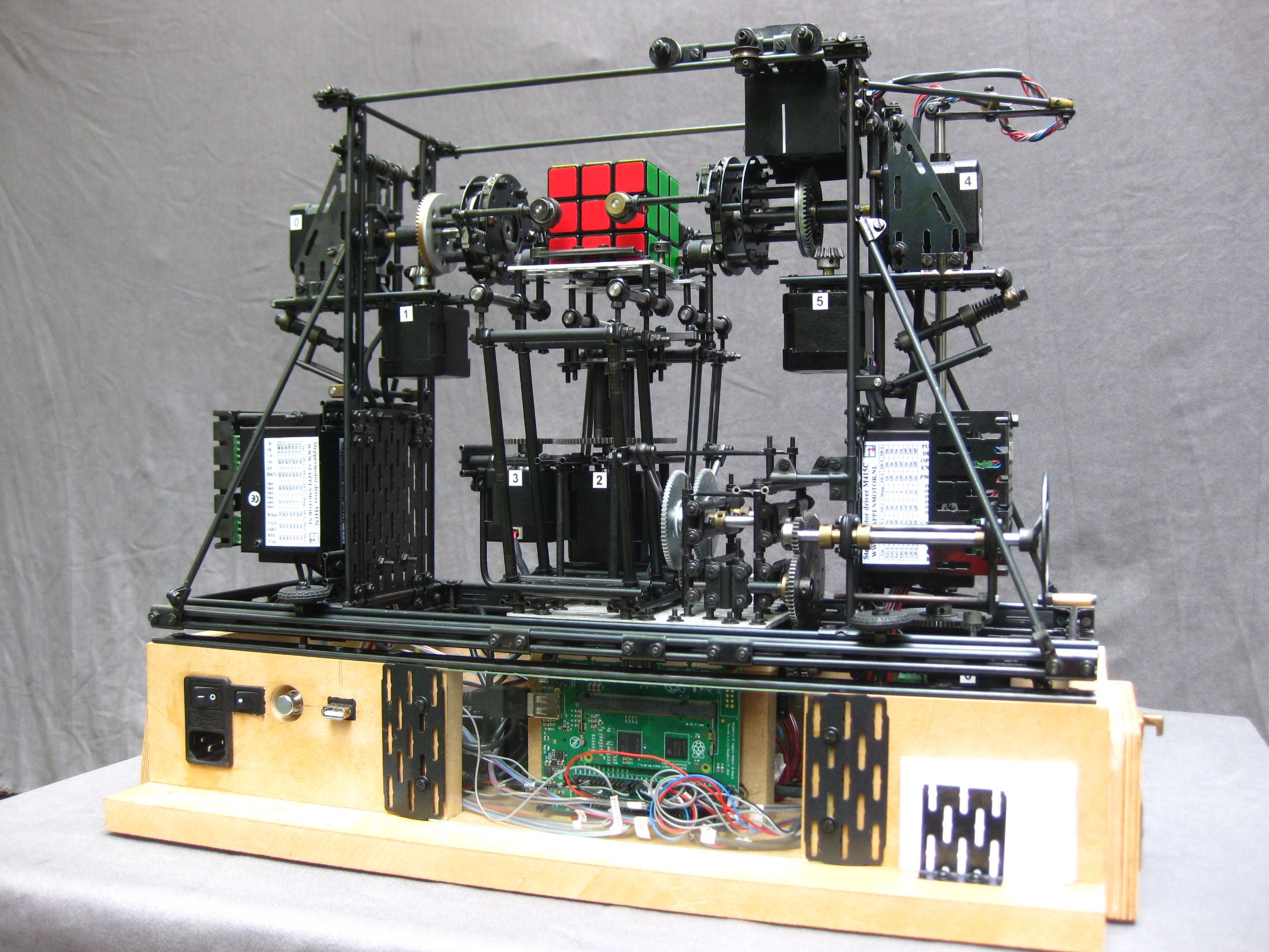
Hardware
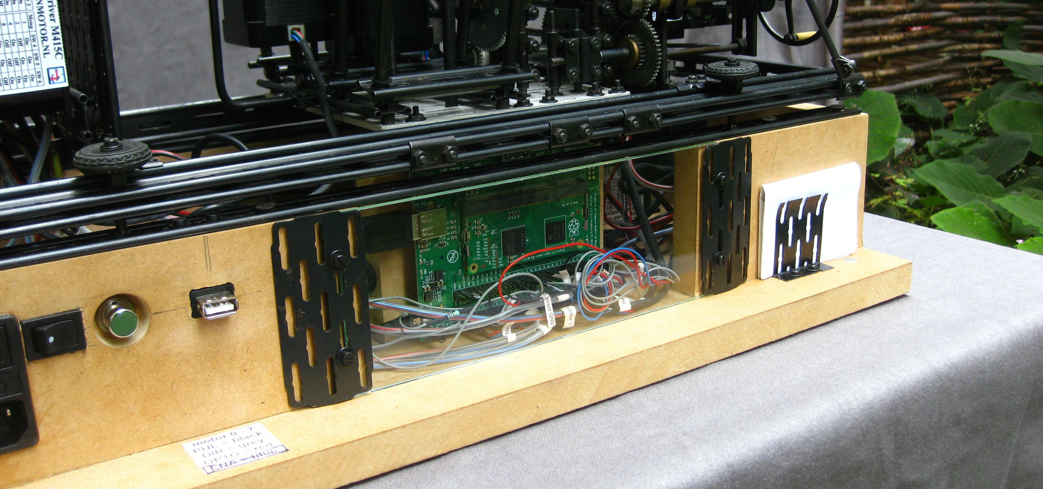
Main board
First of all, we decided to replace Arduino board with Raspberry Pi. This was for a number of reasons: it seemed that we didn’t really need low-level capabilities of Arduino, and I didn’t feel like writing everything in the limited dialect of C++ used by Arduino. Moreover, sophisticated cube solving algorithms required quite a lot of memory, that Arduino cannot provide.
The standard version of Raspberry Pi did not have enough GPIO pins, so we got a Compute Module Development Kit. That one is really cool: not only it has a way more convenient pinout with 45 controllable pins, but it also has two camera slots. We were so happy with it that we bought two more boards for future projects :)
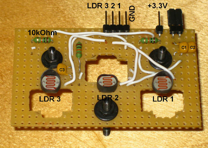
Capacitor-based scanner
Of course, this change from Arduino to Raspberry required some changes in circuits as well. One of the problems was that you can only get 3.3V from Raspberry’s GPIO pin whereas Arduino gives you 5V. Fortunately, our motor drivers still worked under lower voltage, so we only needed to change resistors in scanner circuit.
Much more annoying problem was that Raspberry didn’t have analog input. This was crucial for us because our color scanner was based on LDRs. On Arduino, it was very easy to read the value from LDR, but to do the same in Raspberry one has to use external devices or make some hacks. After all, we took this approach. Basically, instead of reading the voltage, we are counting the time needed to charge the capacitor. This time is proportional to LDR resistance, so in the end we can estimate its value.
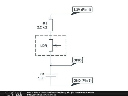
Of course, it was not reliable. Mainly, because there are a lot of background processes running alongside your program on Raspberry, so you always get random deviations in readings. This is not so important if you just need to detect the light with LDR, but can have nasty consequences if you want to compare the amounts of light. To circumvent this effect, we had to do multiple readings every time, detect outliers, and calculate an average between the remaining values.
Here is the video of a machine with capacitor-based scanner:
Arduino-controlled scanner
Though we made the capacitor-based scheme working, it was ridiculously slow. It would take about two minutes to scan the whole cube. So we decided to get a small Arduino board specifically to control the scanner.
It turned out to be very easy to connect Arduino to Raspberry and make them work together. We only needed two wires, this tiny little level converter in between - and voila: we have a serial connection between the boards. I also used cool Min protocol on top of serial to make it more convenient.
This change dramatically decreased the time required for scanning the cube. Since Arduino can read the voltage directly from the LDR, we don’t need to wait until capacitor is charged, and we don’t need to do it multiple times anymore!
Solving algorithm
The most important part of the solving program is a solving algorithm. There is quite some serious mathematical work already done on Rubik’s cube. If you are into algebra and combinatorics, it might be pretty interesting. For instance, I was very surprised that the God number (the exact lower bound for a number of moves needed to solve arbitrary cube) was only found in 2010!
While we did care about the speed of solving, we had to take into account that Raspberry Pi has limited computational powers. Therefore, we could not use the optimal solver as it would require a lot of time for bruteforcing. After all, we ended up with a great two-phase algorithm by Herbert Kociemba.
The original implementation of the two-phase algorithm is only available in Java. First thing I did was translating it to Python. It turned out to be quite easy and straightforward. However, in the beginning I didn’t realize that solving the Rubik’s cube requires a lot of resources. When I first started Python solver, it took about one minute (!) to find a solution on my MacBook.
PyPy showed much better results, it reduced the time to one second on the laptop, but it was still about a minute on Raspberry. After a day trying different ways to speed up Python code, I decided to go for a pure C version. This solved all problems: now it takes about one second to find a solution, even on Raspberry Pi. This was good enough for this project.
I have published both Python and C versions of the solver on GitHub.
Moving the assembly
Next step was to build a program that would actually control the machine. This implied moving the motors, carefully handling gear ratios, keeping in mind the limitations forced by the assembly (for example, side grippers can only be rotated when the bottom gripper is in certain position). Some additional code was required to handle user input (machine has a multi-purpose controlling button), and to optimize gripper movements. All in all, there was nothing special in this part, just a routine software development.
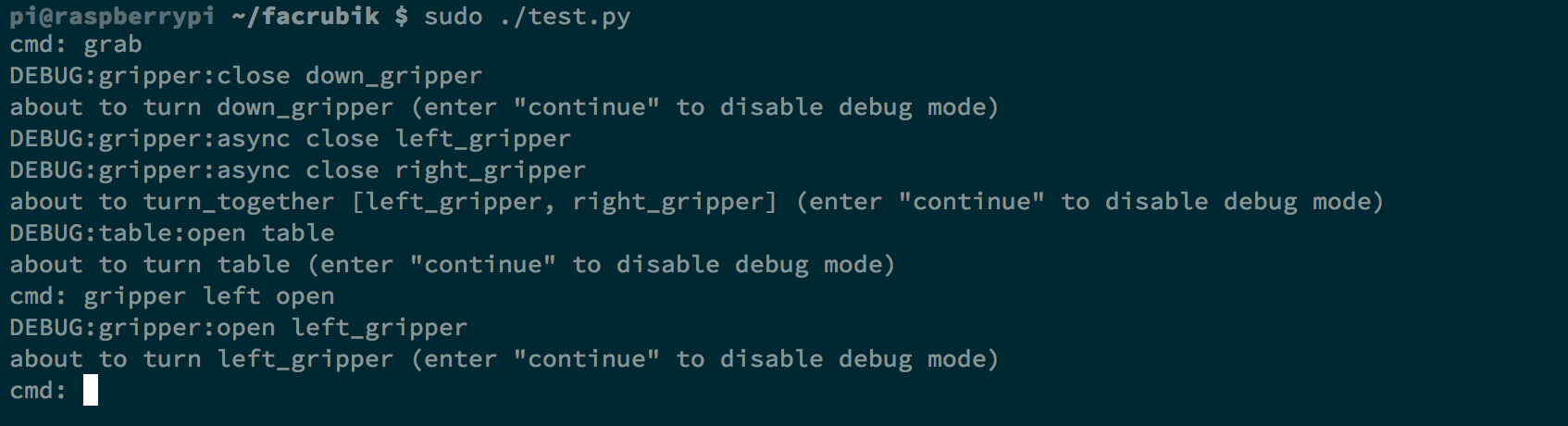
I also made a handy interactive shell for debugging purposes. It made testing very convenient and I could easily debug parts of the program. To debug the scanning, I rendered nice images to visualize the readings.
Scanning and color recognition (a.k.a. devil in details)
Update: This section describes the previous version of the scanner (capacitor-based). New Arduino-controlled scanner made the readings much more reliable and fast. However, color clustering algorithm remained the same.
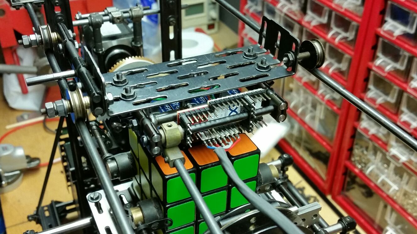
Up to this point, things were exciting, but not difficult. And we were ready to open champagne to celebrate our great success. The only thing left was to recognize the colors using an LDR-based scanner. The idea was as simple as it could be: we had 3 sets of LEDs (red, green, and blue) which we turned on one by one and captured reflected light with LDRs. Essentially, this gave us RGB values which we could use for color recognition. We already had a proof-of-concept program which seemed to work well on Arduino, so we didn’t expect surprises here.
However, the scanning process turned out to be the most challenging part of the whole project. It took almost 2 months to accomplish this.
Problems
First of all, we had to fundamentally change the circuit of the scanner, as described above.
Due to the hack with capacitors, it introduced random errors in our readings. So the first thing was to do several readings in a row and get rid of outliers. Once we did that, we could get something like following (these are results of scanning a solved cube in a dark room):
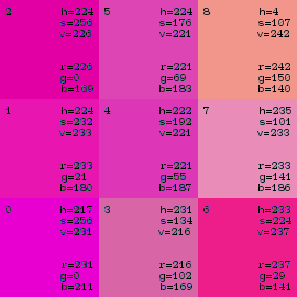
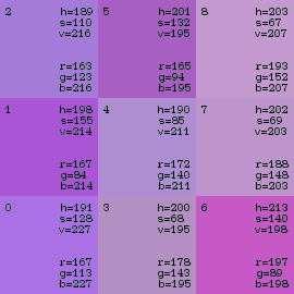
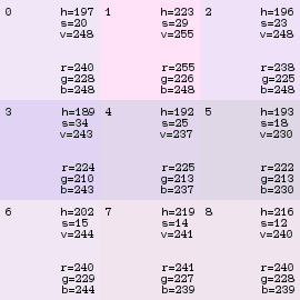
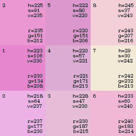
As you can see, this is far from ideal. First, results for the same color in different positions significantly differ due to the fact that every LDR and every LED is pointing in a slightly different direction. Second, sometimes different colors can have overlapping value ranges (for example, red and orange often appear the same). Finally, all the readings are highly sensitive to the ambient light.
Due to the random deviation in readings and ambient light, dispersion is quite extensive as seen on the following (clickable) plot (by the way, you should check out plot.ly, it is awesome):

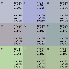
UPD: Arduino-based scanner showed much better results:

Clustering color values
Given these results, I came up with two fundamentally different approaches to color recognition:
1. Color ranging
Find the ranges (a cubical region in RGB color space) for each color and just look for a suitable range every time we scan a facelet. Each combination of facelet position, LDR, and LED color should be handled separately. While this approach is quite straightforward and easy to implement, we have to stick to particular cube colors. And in the end it turned out to be not usable under different ambient light conditions since some ranges overlap and, therefore, become ambiguous.
2. True clustering
Make artificial tweaks on raw values to make the same colors in different positions look similar. If we can do this, we can apply some clustering algorithm to distinguish colors. The most difficult part here was to figure out proper tweaking coefficients that would work well under different circumstances and ambient conditions. Unfortunately, this approach was not usable as well, due to probability nature of clustering algorithms: they are mostly intended to give a “decent” solution, but not the exact one.
Compromise
Each of the approaches above has its pros and cons. So after all we used a sort of a mixed algorithm:
- we do some artificial calibrations based on gathered statistics to normalize the readings
- convert values from RGB to HSV
- find a white cluster, by taking out 9 facelets with the least Saturation
- artificially increase saturation for all other facelets
- do a simple clustering of remaining (non-white) colors by comparing to center facelets
Ambient light elimination
Even with a decent clustering algorithm, scanning was still tricky due to the ambient light. What seemed to work perfectly in a dark room, failed miserably under a bright sun, and vice versa. So the final step was to get rid of the ambient light. Wilbert had to do quite some work on the scanner module to isolate LDRs from ambient light. It took 3 iterations: each time we thought it was ready, but each time we would find another hole through which ambient light could reach the LDRs:
Summary and promises
This project was fun. It was very exciting to bring it to life step by step, and such a pleasure to see it working after we put so much effort in it. But this is nothing compared to how much we learned thanks to it. What seemed to be pretty easy from the beginning, turned out to be very tricky in details. I could not imagine I would have to learn statistical methods and clustering algorithms, dust off my school notes on electronics (though we only need the basics here), and discover a number of useful tools and services along the way. This is why I am so happy I had a chance to work on this.
That said, this machine was only a prototype. We didn’t contemplate to challenge record-breaking robots in terms of solving speed, and we didn’t really make the most of the hardware parts. But we will definitely go for it in the next generation of this machine.